Over the last two decades, the computer vision community has witnessed extensive research in the area of analyzing and understanding scenes containing different moving objects (usually referred ad dynamic scenes). Motion segmentation forms a significant part of this analysis and deals with separating into different groups some visual features extracted from these scenes, such that each group corresponds to a different motion.
Based on what type of visual features are extracted, the research in motion segmentation can be broadly divided into two categories. The first one is termed as direct motion segmentation and uses the intensities from the image of a scene in order to perform segmentation. This genre of algorithms separates the images into different patches that have the same 2-D motion, i.e. apparent motion in the images. The second category of algorithms proceeds by segmenting a sparse set of features corresponding to actual physical points on the objects. These features can be used to characterize either the 2-D motion of the scene or the 3-D motion of the objects imaged in the scene.
In our research, we have developed a general algebraic approach which can handle both types of features from two views in a unified manner.
Our latest research aims to solve the motion segmentation problem in the case where multiple-view point correspondances are available.
In direct motion segmentation, the spatial-temporal derivatives of the image intensities help us solve the segmentation problem. In the case of pixels that obey a single 2-D translational motion, these derivatives constitute a linear subspace. In the case of pixels that obey a sing 2-D affine motion, these derivatives along with the pixel co-ordinates constitute a bilinear subspace. When the scene contains only translational motions or only affine motions, the segmentation problem reduces to one of separating linear subspaces or bilinear subspaces respectively. However, when the scene contains both kind of motions, the problem becomes one of separating linear and bilinear subspaces.
Most of the existing algorithms perform 2-D motion segmentation by assuming that the motions in the scene can be modeled by 2-D affine motion models. In theory, this is valid because the simpler 2-D translational motion model can be represented by the more general affine motion model. However, such approximations in modeling can have negative consequences. Firstly, the translational model has 2 parameters and the affine model has 6 parameters. Therefore, for each translational model in the scene, the approximation in modeling leads to the estimation of 4 extra parameters. Moreover, since the data might not be rich enough to estimate the affine motion model, the parameter estimation might be erroneous. In our research, we address the problem of segmenting scenes that contain translational motion models as well as affine motion models without making any approximations in modeling the motions of the scene.
Our method is algebraic in nature and proceeds by fitting a polynomial to the image data such that it is satisfied by all the measurements irrespective of their true grouping. The polynomial helps characterize the vanishing set of the union of the individual linear and bilinear subspaces. Since this polynomial is representative of the individual motion models, it helps us define a Multibody Brightness Constancy Constraint (MBCC). The MBCC is essentially a homogeneous polynomial in the image derivatives and pixel co-ordinates, and forms the backbone of our proposed solution. A 3x3 sub-matrix of the MBCC's hessian when evaluated at the image measurements corresponding to a pixel, helps us identify the type of motion model at the pixel. This identification essentially involves a rank check of 1 vs 3 for checking if the type of motion model is 2-D translational or 2-D affine. Once the type of motion models are identified, the algorithm uses the first order derivatives of the MBCC and their cross products to estimate the individual motion models. After estimating the motion models, we perform segmentation by assigning to each pixel the motion model that explains its motion the best. While our method has the novelty of being the first known algebraic approach to account for the different kinds of models, it also has an important theoretical contribution shows that algebraic methods of similar nature as ours would fail if an translational model is approximated by an affine motion model.
The following is a typical example of demonstrating the power of our algorithm. The scene contains one 2-D translational motion(background patch in brown) and one 2-D affine motion model(foreground patch in blue). Fitting two 2-D translational motion models obviously gives poor segmentation results since the scene is not explained comprehensively. Similarly, fitting two affine motion models gives rise to a degeneracy and the algebraic segmentation algorithm breaks down. However, when we fit one 2-D translational model and one 2-D affine model, the correct segmentation results are obtained. The results show attempts to segment the background and the pixels that do not belong to the group are marked in black.
|
|
|
|
|||
|
|
|
|
|||
Frames from original sequence |
Segmentation of background | Segmentation of background | Segmentation of backgroundi |
In many areas of dynamic scene understanding, we are dealing with features that corresponds to actual 3-D points in the scene. We can use a tracker to extract these features, looking for points that present particular appareance characteristics (e.g., one can use intensity corners or SIFT features).
As we have said, each feature corresponds to a 3-D point in the scene. We refer to the set of all the images of the same point from all the frames as a trajectory. Then, the multibody motion segmentation problem can be defined as the task of clustering the point trajectories.
In general, the nature of the solution to this problem heavily depends on the nature of the camera model we assume (essentialy, the camera model specifies how the 3-D points translate in image points in each frame). In our research, we have proposed different solutions for two of the camera models most popular in the literature (affine and perspective).
The algorithms that we are going to present below assume that the feature points are visible in all the frames (also called views). However, there are techniques ([8],[9]) which can extend the existing methods to the case of missing data (where some of the features are not visible in all the frames). We refer the reader to the cited paper for more details on this specific topic.
Each column of W corresponds to the trajectory of a point and is represented by a vector in R2F.
It can be shown that under the assumptions given above, the matrix W can be factorized and that the trajectories of points corresponding to the same object lie on a linear subspace of dimension at most four in R2F. Consequently, the problem of motion segmentation can reduced to a subspace separation problem, for which different solutions have already been proposed in the literature.
In our research we analyzed the solutions obtained using GPCA (Generalized PCA) and LSA (Local Subspace Analysis). Both approaches are algebraic in nature but they differ in the fact that the former is global while the second is local. More precisely, GPCA fits a single multibody model using all the data points (trajectories) at the same time and then the data is clustered according to this model. On the other hand, LSA locally fits a low dimensional subspace to each point and its neighbour and then exploits a similarity measure between these local estimation to perform the clustering task.
We compared these two solution to other state-of-the-art techniques using our Hopkins 155 dataset. A small summary of the results can be found at the end of the page while a more comprehensive analysis can be found in the references.
Under the perspective projection model, the relation between points and images is given by
We can note that if the depths were known, one could rescale the entries of W accordingly and the segmentation problem would reduce to the affine projection case (see previous section). On the other hand, if the segmentation was given, one could use standard Structure from Motion (SfM) techniques on each group to recover the depths.
Our proposed algorithm iterates between these two steps (segmentation and depth computation), starting with an estimation of either the segmetation or the depths and terminating when convergence to a stable solution is obtained. Variations of this algorithm can be obtained by mixing different types of initialization and different solutions (GPCA or LSA) for the segmentation step. We again used the Hopkins 155 dataset to compare the performances of our algorithm with the state-of-the-art. Some of the results can be found at the end of the page, while a more thorough analysis can be found in the references.
In addition to the techniques mentioned above, we have developed an extremely general motion segmentation algorithm that can deal with all kinds of motions (full tri-dimensional, planar, homographies, etc.) under the same framework. In fact, motion segmentation is just an application of the more general algorithm devised for unsupervised manifold clustering, a detailed description of which can be found here. Inspired by the Linearly Local Embedding (LLE) algorithm, we use local embedding techniques to solve the segmentation problem. In short, each point is represented as a linear combination of its neighbour. The weights of the linear combination are used to build a similarity matrix, whose eigenvectors encode the desired segmentation.
To compare the performance of the different solutions for segmenting feature trajectories, we developed the Hopkins-155 dataset, a collection of 155 videos containing two or three moving rigid objects. You can follow the link to obtain more specific information on the dataset.
Checker. | GPCA | LSA 5 | LSA 4n | MSL | RANSAC | DI-GPCA | DI-LSA | SI-GPCA | SI-LSA | LLMC 5 | LLMC 4n | CCS | ALC 5 | ALC sp | SSC |
---|---|---|---|---|---|---|---|---|---|---|---|---|---|---|---|
Average | 6.09% | 8.84% | 2.57% | 4.46% | 6.52% | 4.29% | 2.86% | 4.18% | 2.61% | 4.37% | 4.65% | 16.37% | 2.56% | 1.49% | 1.12% |
Median | 1.03% | 3.43% | 0.27% | 0.00% | 1.75% | 2.09% | 0.25% | 2.24% | 0.42% | 0.00% | 0.11% | 10.64% | 0.00% | 0.27% | 0.00% |
Traffic | GPCA | LSA 5 | LSA 4n | MSL | RANSAC | DI-GPCA | DI-LSA | SI-GPCA | SI-LSA | LLMC 5 | LLMC 4n | CCS | ALC 5 | ALC sp | SSC |
Average | 1.41% | 2.15% | 5.43% | 2.23% | 2.55% | 0.52% | 5.74% | 0.65% | 4.54% | 0.84% | 3.65% | 5.27% | 2.83% | 1.75% | 0.02% |
Median | 0.00% | 1.00% | 1.48% | 0.00% | 0.21% | 0.00% | 1.55% | 0.00% | 1.30% | 0.00% | 0.33% | 0.00% | 0.30% | 1.51% | 0.00% |
Other | GPCA | LSA 5 | LSA 4n | MSL | RANSAC | DI-GPCA | DI-LSA | SI-GPCA | SI-LSA | LLMC 5 | LLMC 4n | CCS | ALC 5 | ALC sp | SSC |
Average | 2.88% | 4.66% | 4.10% | 7.23% | 7.25% | 4.79% | 7.95% | 4.55% | 4.38% | 6.16% | 5.23% | 17.58% | 6.90% | 10.70% | 0.62% |
Median | 0.00% | 1.28% | 1.22% | 0.00% | 2.64% | 0.43% | 1.39% | 0.43% | 1.39% | 1.37% | 1.30% | 7.07% | 0.89% | 0.95% | 0.00% |
All | GPCA | LSA 5 | LSA 4n | MSL | RANSAC | DI-GPCA | DI-LSA | SI-GPCA | SI-LSA | LLMC 5 | LLMC 4n | CCS | ALC 5 | ALC sp | SSC |
Average | 4.59% | 6.73% | 3.45% | 4.14% | 5.56% | 3.36% | 4.07% | 3.30% | 3.27% | 3.62% | 4.44% | 12.16% | 3.03% | 2.40% | 0.82% |
Median | 0.38% | 1.99% | 0.59% | 0.00% | 1.18% | 0.59% | 0.51% | 0.53% | 0.53% | 0.00% | 0.24% | 0.00% | 0.00% | 0.43% | 0.00% |
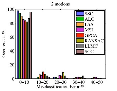
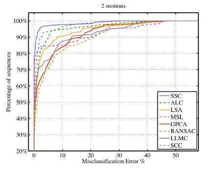
Histograms and cumulative distributions of the errors per sequence |
Checker. | GPCA | LSA 5 | LSA 4n | MSL | RANSAC | DI-GPCA | DI-LSA | SI-GPCA | SI-LSA | LLMC 5 | LLMC 4n | CCS | ALC 5 | ALC sp | SSC |
---|---|---|---|---|---|---|---|---|---|---|---|---|---|---|---|
Average | 31.95% | 30.37% | 5.80% | 10.38% | 25.78% | 20.54% | 6.67% | 22.44% | 5.55% | 10.70% | 12.01% | 28.63% | 6.78% | 5.00% | 2.97% |
Median | 32.93% | 31.98% | 1.77% | 4.61% | 26.01% | 17.30% | 1.00% | 23.20% | 1.21% | 9.21% | 9.22% | 33.21% | 0.92% | 0.66% | 0.27% |
Traffic | GPCA | LSA 5 | LSA 4n | MSL | RANSAC | DI-GPCA | DI-LSA | SI-GPCA | SI-LSA | LLMC 5 | LLMC 4n | CCS | ALC 5 | ALC sp | SSC |
Average | 19.83% | 27.02% | 25.07% | 1.80% | 12.83% | 2.46% | 10.21% | 8.00% | 9.51% | 2.91% | 7.79% | 3.02% | 4.01% | 8.86% | 0.58% |
Median | 19.55% | 34.01% | 23.79% | 0.00% | 11.45% | 0.55% | 4.71% | 2.06% | 4.71% | 0.00% | 5.47% | 0.18% | 1.35% | 0.51% | 0.00% |
Other | GPCA | LSA 5 | LSA 4n | MSL | RANSAC | DI-GPCA | DI-LSA | SI-GPCA | SI-LSA | LLMC 5 | LLMC 4n | CCS | ALC 5 | ALC sp | SSC |
Average | 16.85% | 23.11% | 7.25% | 2.71% | 21.38% | 6.72% | 2.13% | 7.05% | 3.52% | 5.60% | 9.38% | 44.89% | 7.25% | 21.08% | 1.42% |
Median | 28.66% | 23.11% | 7.25% | 2.71% | 21.38% | 6.72% | 2.13% | 7.05% | 3.52% | 5.60% | 9.38% | 44.89% | 7.25% | 21.08% | 0.00% |
All | GPCA | LSA 5 | LSA 4n | MSL | RANSAC | DI-GPCA | DI-LSA | SI-GPCA | SI-LSA | LLMC 5 | LLMC 4n | CCS | ALC 5 | ALC sp | SSC |
Average | 28.66% | 29.28% | 9.73% | 8.23% | 22.94% | 18.38% | 10.89% | 17.50% | 9.77% | 8.85% | 11.02% | 26.18% | 6.26% | 6.69% | 2.45% |
Median | 28.26% | 31.63% | 2.33% | 1.76% | 22.03% | 16.11% | 4.04% | 16.74% | 2.33% | 3.19% | 6.81% | 31.74% | 1.02% | 0.67% | 0.20% |
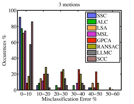
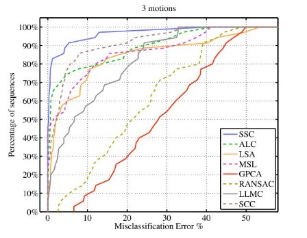
Histograms and cumulative distributions of the errors per sequence |